
I don't know how I feel about these lectures. Oh wait, I do - I don't like them! As someone who doesn't have any experience with AI I have no idea how everyone is understanding what Nathan is saying. What I do know, though, is that his slides are VERY wordy, and writing everything down in my little paper notebook isn't going to work out. Well, I guess another module falls victim to my website. I'm just hoping that it's at least good typing practice.
IMPORTANT!
This site is no longer being updated, as I have moved onto hosting locally. I'm not sure who's reading this, but please contact me on discord at Mushroom#2988 if you need anything.
About
Rational Agents
Inputs to an Agent
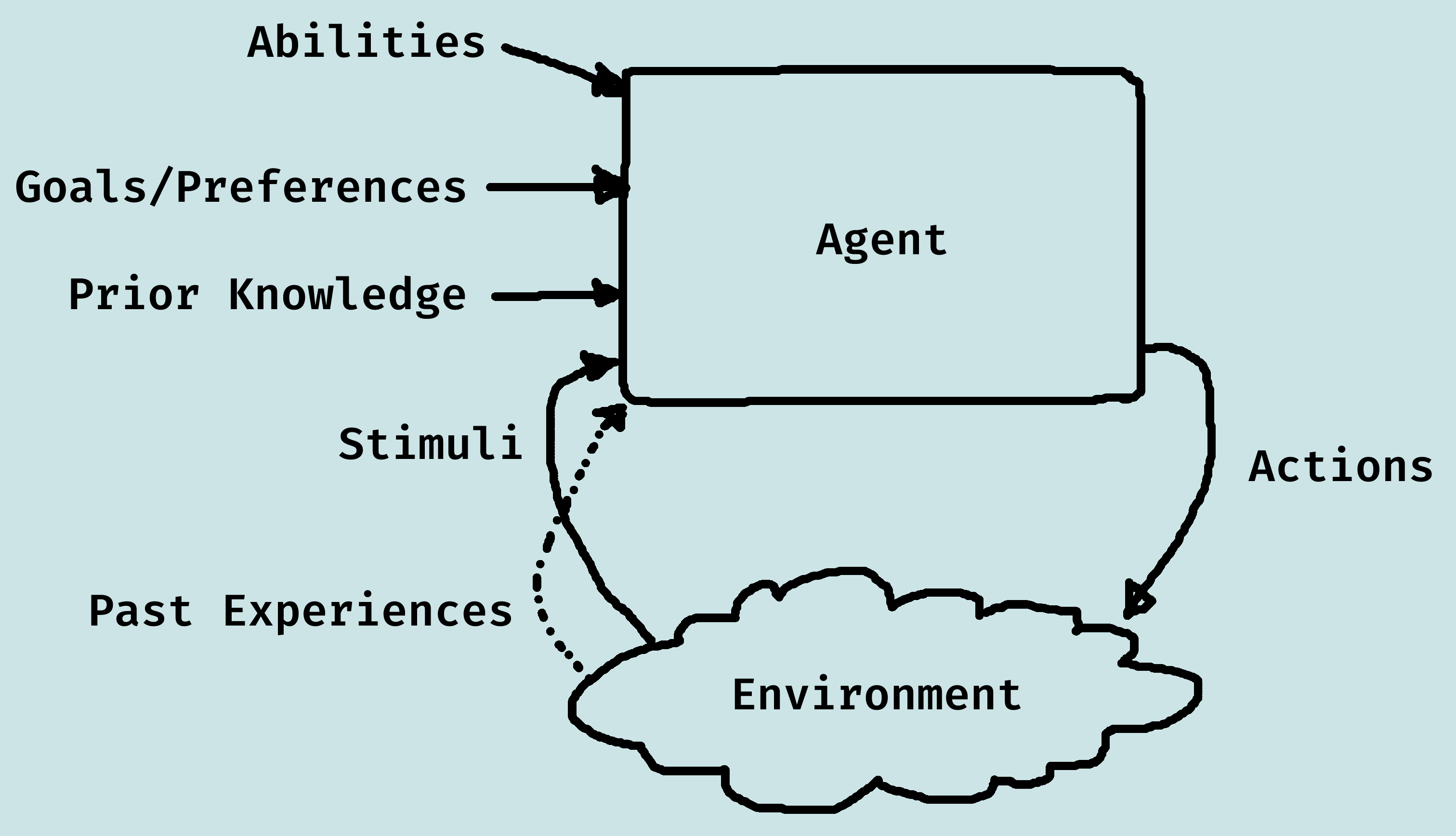
- Abilities: The set of possible actions it can perform.
- Goals/Preferences: What it wants, its values...
- Prior Knowledge: What it comes into being knowing, what it doesn't get from experience...
- History of Stimuli: Current stimuli and past experiences.
Rational Agents
Without loss of generality, "goals" can be specified by some performance measure, defined by a numerical value.
Rational action is whichever action maximises the expected value of the performance measure, given the percept sequence to date (i.e. doing the right thing).
Previous perceptions are typically important.
Remember that rational ≠ omniscient, clairvoyant, or successful.
Dimensions of Complexity
We can view the design space for AI as being defined by a set of dimensions of complexity:
| Dimension | Possible Values |
|---|---|
| Modularity | flat, modular, hierarchical |
| Planning Horizon | non-planning, finite stage, indefinite stage, infinite stage |
| Representation | states, features, relations |
| Computational Limits | perfect rationality, bounded rationality |
| Learning | knowledge is given, knowledge is learned |
| Sensing Uncertainty | fully observable, partially observable |
| Effect Uncertainty | deterministic, stochastic |
| Preference | goals, complex preferences |
| Number of Agents | single agent, multiple agents |
| Interaction | offline, online |
Modularity
- Agent structure has one level of abstraction: flat
- Agent structure has interacting modules that can be understood separately: modular
- Agent structure has modules that are (recursively) decomposed into modules: hierarchical
- Flat representations are adequate for simple systems
- Complex biological systems, computer systems, organizations are all hierarchical
- A flat description is either continuous or discrete. Hierarchical reasoning is often a hybrid of continuous and discrete.
Planning Horizon
The planning horizon is how far the agent looks into the future when deciding what to do.
- Static: world does not change.
- Finite Stage: agent reasons about a fixed finite number of time steps.
- Indefinite Stage: agent reasons abouta finite, but not predetermined, number of time steps.
- Infinite Stage: agent plans for going on forever (process oriented).
Representation
Much of modern AI is about finding compact representations and exploiting the compactness for computational gains. An agent can reason in terms of:
- Explicit States: a state is one way the world could be.
- Features/Propositions: states can be described using features.
- Individuals & Relations: there is a feature for each relationship on each tuple of individuals. Often an agent can reason without knowing the individuals or when there are infinitely many individuals.
Computational Limits
- Perfect Rationality: the agent can determine the best course of actions, without taking into account its limited computational resources.
- Bounded Rationality: the agent must make good decisions based on its perceptual, computational and memory limitations.
Learning From Experience
Whether the model is fully specified a priori:
- Knowledge is given.
- Knowledge is learned form data or past experience.
This is usually a mix of prior knowledge and learning.
Sensing Uncertainty
There are two dimensions for uncertainty: sensing and effect. In each dimension an agent can have:
- No uncertainty: the agent knows what is true.
- Disjunctive uncertainty: there is a set of states that are possible.
- Probabilistic uncertainty: a probability distribution over the worlds.
For sensing uncertainty, whether an agent can determine the state from its stimuli:
- Fully-observable: the agent can observe the state of the world.
- Partially-observable: there can be a number of states that are possible given the agent's stimuli.
Effect Uncertainty
If an agent knew the initial state and its action, could it predic the resulting state? The dynamics can be:
- Deterministic: the resulting state is determined from the action and the state.
- Stochastic: there is uncertainty about the resulting state.
Preferences
What does the agent try to achieve?
- Achievement goal is a goal to achieve - this can be a complex logical formula.
- Complex preferences may involve tradeoffs between various desiderata, perhaps at different times. (Ordinal: only the order matters; Cardinal: absolute values also matter.)
Number of Agents
Are there multiple reasoning agent that need to be taken into account?
- Single agent reasoning: any other agents are part of the environment.
- Multiple agent reasoning: an agent reasons strategically about the reasoning of ther agents.
Agents can have their own goals: cooperative, competitive, or goals can be independent of each other.
Interaction
When does the agent reason to determine what to do?
- Reason offline: before acting.
- Reason online: while interacting with the environment.
Representations
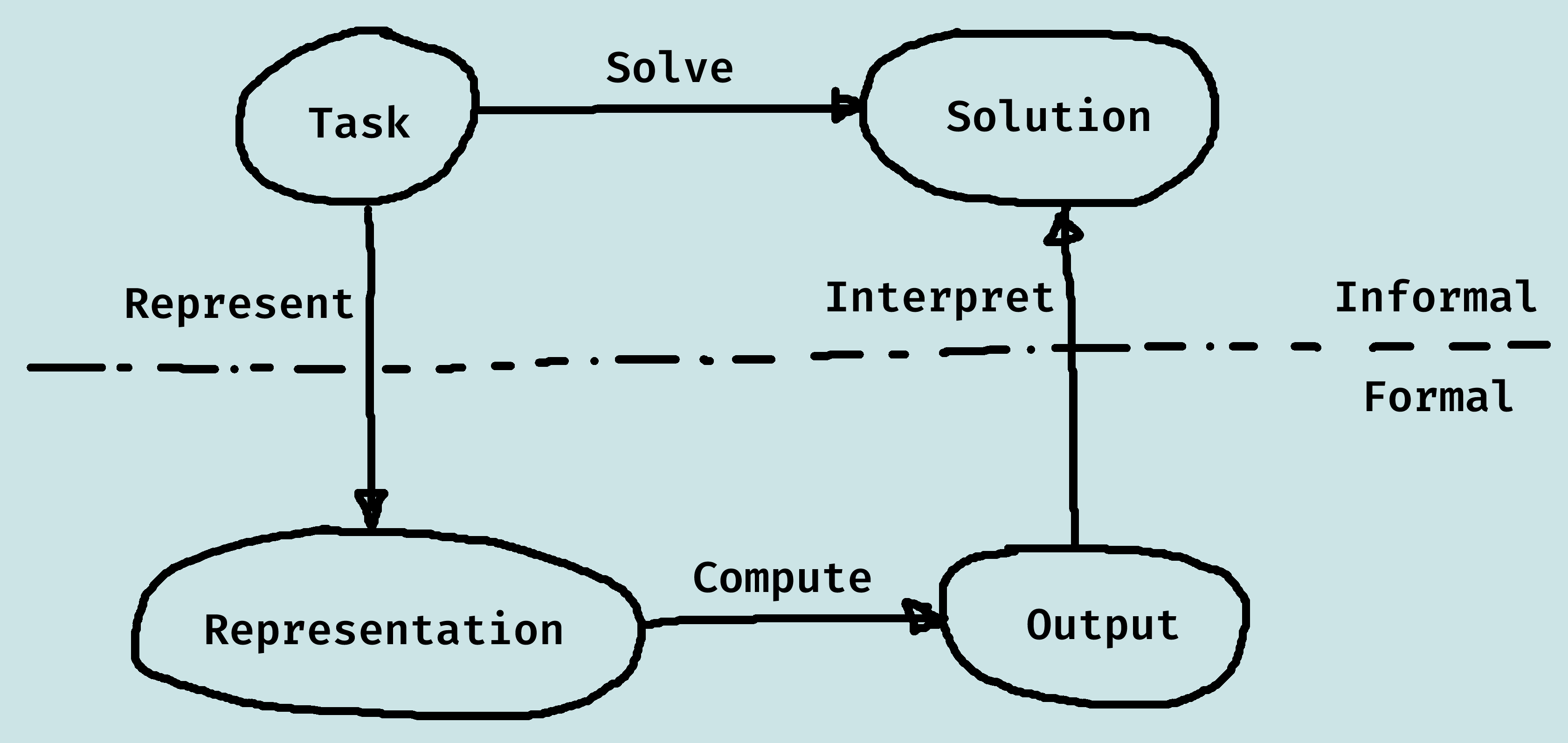
We want a representation to be:
- Rich enough to express the knowledge needed to solve the problem.
- As close to the problem as possible: compact, natural and maintainable.
- Amenable to efficient computation (able to trade off accuracy and computation time/space).
- Able to be acquired from people, data and past experiences.
Solutions
Classes of solution:
- An optimal solution is a best solution according to some measure of solution quality.
- A satisficing solution is one that is good enough, according to some description of which solutions are adequate.
- An approximately optimal solution is one whose measure of quality is close to the best theoretically possible.
- A probable solution is one that is likely to be a solution.
Decisions and Outcomes
Good decisions can hav ebad outcomes; bad decisions can have good outcomes.
Information can be valuable because it leads to better decisions.
We can often trade off computation time and solution quality; an anytime algorithm can provide a solution at any time, given more time it can produce better solutions.
An agent is not just concerned about finding the right answer, but about acquiring the approprite information, and computing it in a timely manner.
Agent Architectures and Hierarchical Control
Agents
An agent is something that acts in an environment. It can be a person, a robot, a lamp, or a rat.
Agents interact with the environment with a body. An embodied agent has a physical body.
Agents receive information through their sensors, and their actions depend on what information it receives from its sensors.
Agents act in the world throught their actuators, also called effectors. Note that sensors and actuators can be noisy, unreliable, or broken.
Agent Systems
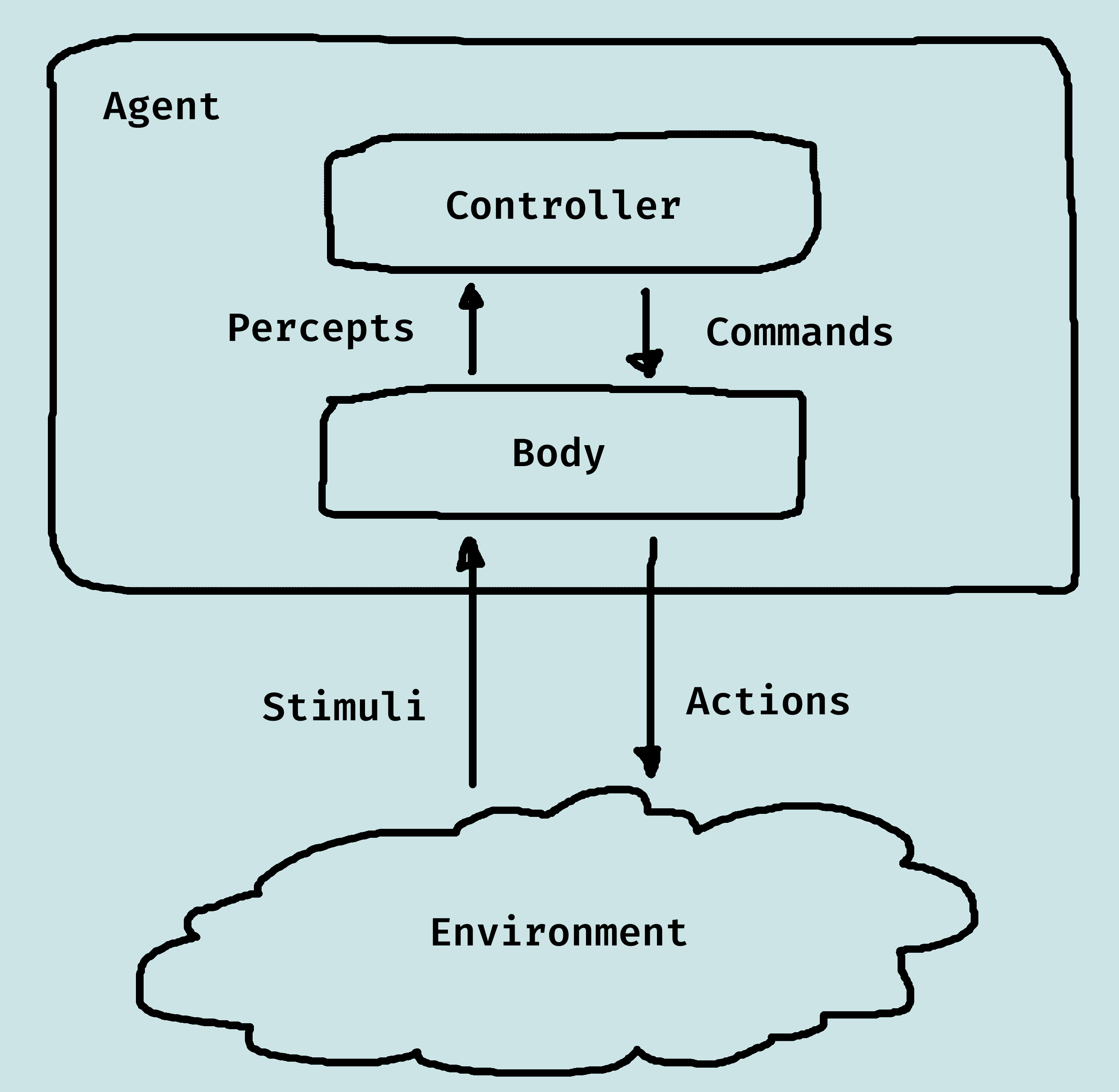
Above is a depiction of the general interaction between an agent and its environment. Together, they are known as the agent system.
The controller receives percepts from the body, and sends commands to the body. The stimuli could be light, sound, certain texts, physical bumps, etc.
Controllers have memory and computational capabilities, albeit both are limited.
The Agent Functions
- A percept trace is a sequence of all past, present, and future percepts received by the controller.
- A command trace is a sequence of all past, present, and future commands output by the controller.
- A transduction is a function from percept traces into command traces.
- A transduction is causal if the command trace up to time t depends only on percepts up to t.
- A controller is an implementation of a casual transduction.
- An agent's history at time t is a sequence of past and preesnt percepts and past commands.
- A causal transduction specifies a function from an agent's history at time t into its action at time t.
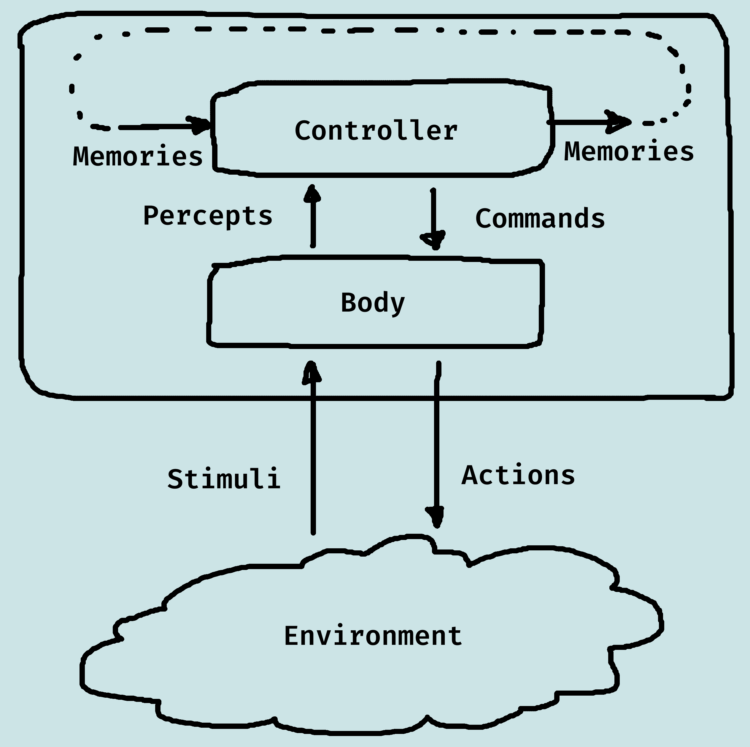
Belief States
An agent does not have access to its entire history, it only has access to what it has remembered.
The memory or belief state of an agent at time t encodes all of the agent's history that it has access to.
The belief state fo an agent encepsulates the information about its past that it can use for current and future actions.
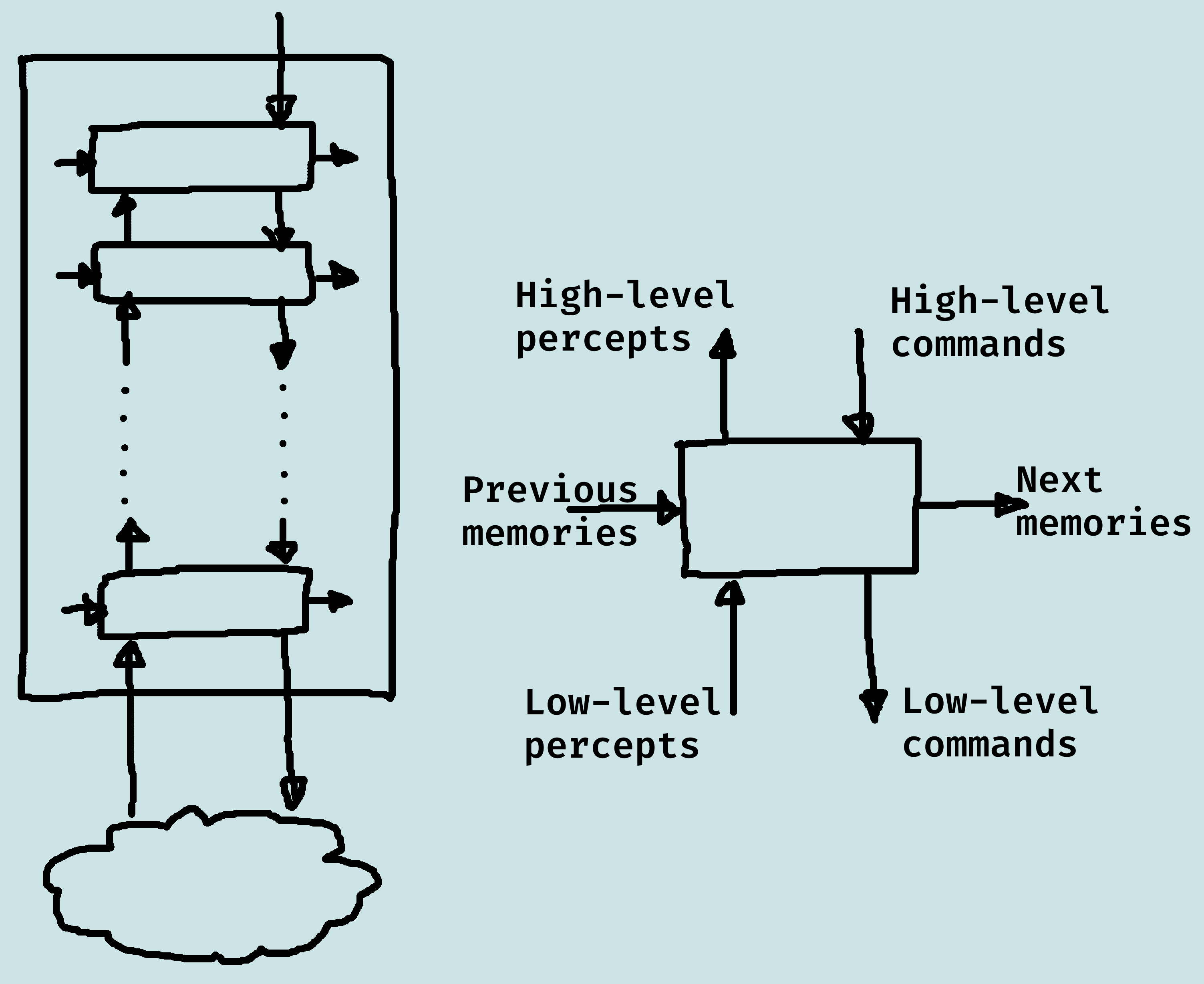
Hiearchical Control
This is an architecture that uses a hierarchy of controllers.
Each controller sees the controllers below it as a virtual body from which it gets precepts and sends commands.
The lower-level controllers can run much faster, and react to the world more quickly, and deliver a simpler view of the world to the higher-level controllers.
Agent Functions
We can view an agent as being specified by the agent function mapping percept sequences to actions f : P → A.
Ideal rational agent: does whatever action is expected to maximise performance measure on basis of percept sequence and built-in knowledge.
So, in principle there is an ideal mapping of percept sequences to actions corresponding to idea agent.
One agent function (or a small equivalence class) is rational (can be seen to approcimate idea mapping).
Aim is to find a way to implement the rational agent function.
There are five fundamental types of agent, i.e. ways of building the agent function, with increasing generality:
- Simple reflex agents: condition-action rules.
- Reflex agents with state: retain knowledge about world.
- Goal-based agents: have representation of what states are desirable.
- Utility-based agents: ability to discern some useful measure between possible means of achieving some state.
- Able to modify their behaviour based on their performance, or in the light of new information.
Reflex Agents
Reflex agents are based on a set of condition-action rules. Although simple, reflex agents can still achieve relatively complex behaviour.
Reflex Agents with State
Pure reflex agents only work if the "correct" decision of what to do can be made on current percept, so we typically need some internal state to track the environment.
The update state function uses knowledge about how the world evolves and how actions affect the world, and the agent can use such information to track unseen parts of the
Goal-based Agents
Knowing current environment state is generally not enough to choose action: need to know WHAT the agent is trying to achieve.
Goal-based agents can combine information about environment, goals, and effects of actions to choose what to do.
This is relatively simple if goal is achievable in a single action, but typically goal achievement needs a sequence of actions.
All in all, a goal-based agent is much more flexible than a reflex agent.
Utility-based Agents
There are typically many ways to achieve a goal. Some results in better utility than the others.
We can use a utility function to judge resulting states of world, and it also enables a choice about which goals to achieve - select the one with highest quality.
If achievement is uncertain we can measure the importance of goal against likelihood of achievement.
Learning Agents
If the designer has incomplete information about the environment, an agent needs to be able to learn.
Learning provides an agent with a degree of autonomy or independence, and percepts can be used to improve agent's ability to act in the future (as well as for choosing an action now).
Learning results from interaction between the agent and the world, and observation by agent of its decision making.
A typical learning agent has four conceptual components:
- Learning element: responsible for making improvements - takes knowledge of the performance element and feedback on agent's success, and suggests improvements to the performance element.
- Performance element: responsible for acting - takes percepts and returns actions. (This would be the whole agent in non-learning agents)
- Critic: tells the learning element how well the agent is doing, using some performance standard.
- Problem generator: responsible for suggesting actions in pursuit of new (and informative) experiences.
Uninformed Search
Problem-Solving
There are four steps a problem-solving agent must take:
- Goal formulation: identity goal given current situation.
- Problem formulation: identify permissible actions (or operators), and states to consider.
- Search: find sequence of actions to achieve goal.
- Execution: perform the actions in the solution.
There are two types of problem-solving:
- Offline: complete knowledge of problem and solution.
- Online: involves acting without complete knowledge of problem and solution.
Problem Types
Deterministic, fully observable → single-state problem.
- Sensors tell agent current state and it knows exactly what its actions do.
- Means that it knows exactly what state it will be in after any action.
Deterministic, partially observable → multiple-state problem.
- Limited access to state, but knows what its actions do.
- Can determine set of states resulting from an action.
- Instead of single states, agent must manipulate sets of states.
Stochastic, partially observable → contigency problem.
- Don't know current state, and don't know what state will result from action.
- Must use sensors during execution.
- Solution is a tree with branches for contigencies.
- Often interleave search and execution.
Unknown state space, i.e. knowledge is learned → exploration problem (online).
- Agent doesn't know what its actions will do.
- Example: don't have a map, get from Coventry to London.
Problem Formulation: State-space Problems
A state-space problem consists of:
- A set of states
- A subset of states called the start states
- A set of actions
- An action function: given a state and an action, returns a new state
- A set of goal states, specified as function, goal(s)
- A criterion that specifies the quality of an acceptable solution.
State space might need to be abstracted for problem solving in the real world.
- Abstract state ≈ set of real states.
- Abstract operators ≈ combination of real actions, e.g. Coventry → Warwick comprises all possible routes, detours, fuel stops etc. (must ensure validity: reliable for all real states in abstract state).
- Abstract solution ≈ set of real paths that are solutions in real world.
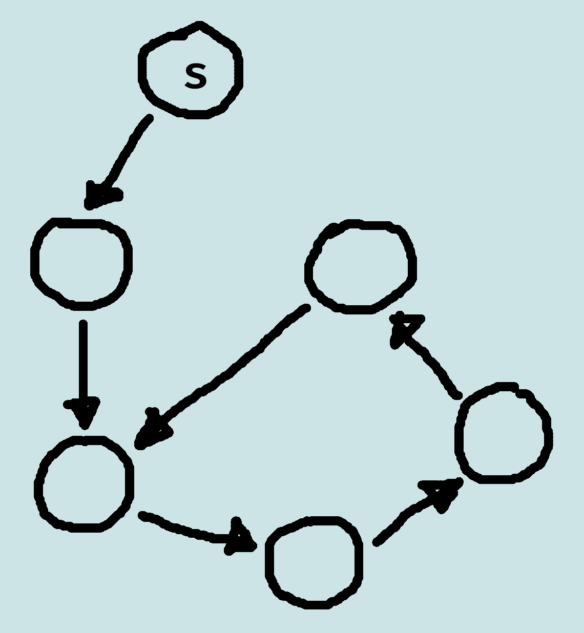
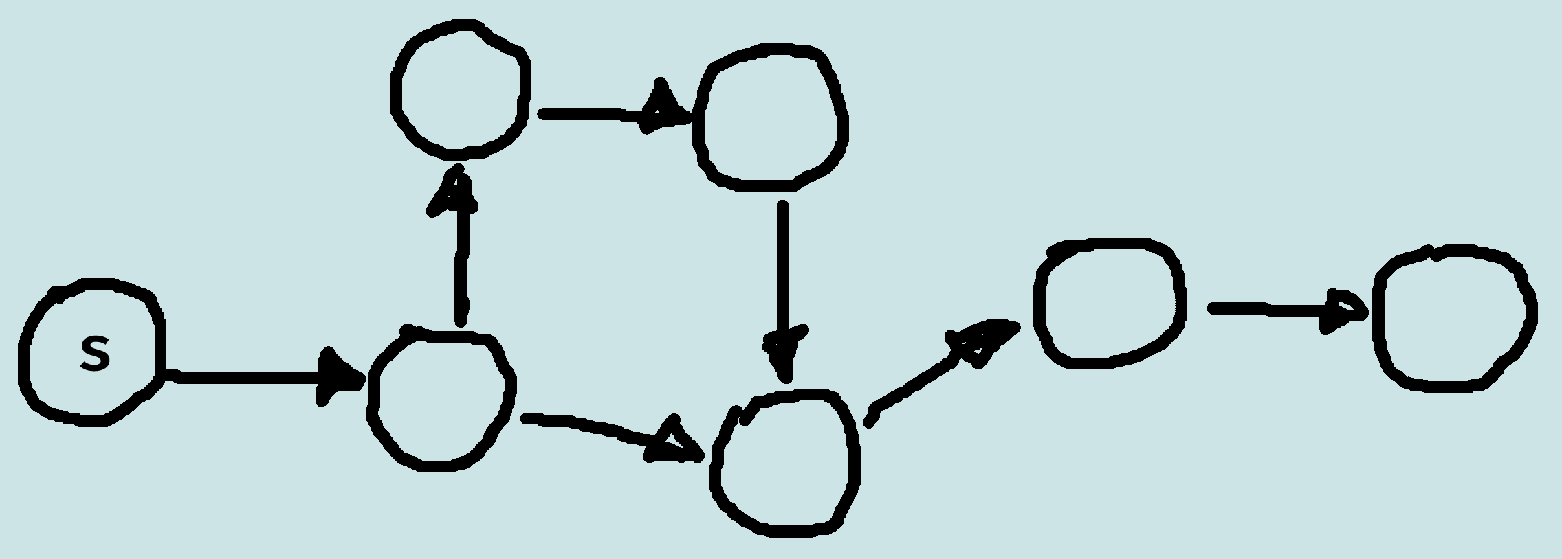
State Space Graphs
A general formulation of a problem solving problem is a state space graph:
- A (directed) graph comprising of a set N of nodes and a set A of ordered pairs of nodes, called arcs or edges.
- Node n2 is a neighbour of n1 if there is an arc from n1 to n2. That is, if (n1, n2) ∈ A.
- A path is a squence of nodes {n0, n1, ... , nk} such that (ni-1, ni) ∈ A.
- The length of a path {n0, n1, ... , nk} is k.
- Given a set of start nodes and goal nodes, a solution is a path from a start node to a goal node.
Tree Search
Tree search is the basic approach to problem solving:
- Offline, simulated exploration of the state space.
- Starting with a start state, expand one of the explored states by generating its successors (i.e. find neighbours by considering possible actions) to build a search tree.
Implementing tree search:
- A state represents a physical configuration.
- A node is a data structure comprising part of search tree.
- A node has: state, parent, children, depth, path cost.
- Nodes waiting to be expanded is called the frontier.
- Represent frontier as a queue.
Tree Search Strategies
We can evaluate strategies along several dimensions:
- Completeness: Always find solution (if it exists)?
- Optimality: Always find a least-cost solution?
-
Time complexity: number of nodes explored?
- Maximum branching factor, b
- Depth of least cost solution, d
- Maximum depth of state space, m (may be ∞)
- Space complexity: maximum number of nodes in memory?
Uninformed search only uses information from problem definition (i.e. we have no measure of the best node to expand). Two simple examples of uninformed search is breadth-first search and depth-first search.
Breadth-First Tree Search
Expand shallowest unexpanded node - put successors at the end of queue (FIFO).
Complete?
- Yes (always finds solution if b is finite).
Time?
- O(bd ).
Space?
- Each leaf node kept in memory: O(bd-1 ) explored and O(bd ) in frontier, so complexity is O(bd ) (i.e. dominated by size of frontier).
Optimal?
- Yes, if cost is nondecreasing function of depth (e.g. operators equal cost); not optimal in general.
Space is the main problem for breadth-first search.
Depth-First Tree Search
Expand deepest unexpanded node - put successors at the front of queue (LIFO).
Complete?
- No. Fails infinite-depth spaces, spaces with loops. Need to modify to avoid repeated states along path.
Time?
- O(bm ). Terrible if m much larger than d. If solutions are dense may be much faster than BFS.
Space?
- O(bm ), i.e. linear space (store path form root to leaf and unexpanded siblings of nodes on path).
Optimal?
- No.
Graph Search
With tree search, state spaces with loops give rise to repeated states that cause inefficiencies, and in fact the complete search tree is infinite.
Graph search is a practical way of exploring the state space that can account for such repetitions.
- Given a graph, start nodes, and goal nodes, incrementally explore paths from the start nodes.
- Maintain a frontier of paths from the start node that have been explored.
- As search proceeds, the frontier expands into the unexplored nodes until a goal node is encountered.
- The way in which the frontier is expanded defines the search strategy.
Breadth-First Graph Search
Treats the frontier as a queue: always selects one of the earliest elements added to the frontier.
If the list of paths on the frontier is [p1, p2, ... , pr ]:
- p1 is selected, and its neighbours are added to the end of the queue, after pr.
- p2 is selected next.
Complete?
- Yes, if the branching factor for all nodes is finite.
Time?
- bn, where b is the branching factor, and n is path length.
Space?
- Exponential in path length: bn.
The search is unconstrained by the goal.
Depth-First Graph Search
Treats the frontier as a stack: always selects one of the last elements added to the frontier.
If the list of paths on the frontier is [p1, p2, ... , pr ]:
- p1 is selected, and the paths that extend p1 are added to the front of the stack (in front of p2 ).
- p2 is only selected when all paths from pi have been explored.
Complete?
- Not guaranteed to halt on infinite graphs, or graphs with cycles.
Time?
- Linear in the number of arcs from the start to the current node.
Space?
- If the graph is a finite tree, with forward branching factor ≤ b and all paths from the start having at most k arcs, worst case time complexity is O(bk ).
The search is unconstrained by the goal.
Lowest-cost-first Search
Sometimes there are costs associated with arcs, and the cost of a path is the sum of the costs of its arcs.
An optimal solution is one with minimum cost.
At each stage, lowest-cost-first search selects a path on the frontier (priority queue ordered by path cost) with lowest cost.
The first path to a goal is a least-cost path to a goal node, and when arc costs are equal just use BFS.
Informed Search
Overview
Uninformed search is generally very inefficient; if we have extra information about the problem, we should use it. This leads to informed search, or heuristic search.
Note that this is still offline problem solving, since we have complete knowledge of problem and solution.
About heuristic search:
- Idea: don't ignore the goal when selecting paths.
- Often there is extra knowledge that can be used to guide the search: heuristics.
- h(n) is an estimate of the cost of the shortest path from node n to a goal node. It needs to be efficient to compute, and it is an underestimate if there is no path from n to a goal with cost (strictly) less than h(n).
- An admissible heuristic is a non-negative heuristic function that is an underestimate of the actual cost of a path to a goal.
Best-first Search
Idea: select the path or node that is closest to a goal according to the heuristic function.
- Heuristic depth-first search selects a neighbour so that the best neighbour is selected first (i.e. appears closest to the goal).
- Greedy best-first search selects a path on the frontier with the lowest heuristic value.
Best-first search treats the frontier as a priority queue ordered by h.
Complete?
- Not guaranteed to find a solution, even if one exists.
Time?
- Exponential in the path length: bn, where b is the branching factor, n is the path length.
Space?
- Exponential in the path length: bn.
Optimal?
- No, it does not always find the shortest path.
A* Search
A* search uses both path cost and heuristic values, where cost(p) is the cost of path p, and h(p) estimates the cost from the end of p to a goal.
A* search is a mix of lowest-cost-first and best-first search. It treats the frontier as a priority queue ordered by f(p), and always selects the node on the frontier with the lowest estimated distance from the start to a goal node constrained to go via that node.
Admissibility of A*
A seearch algorithm is admissible if, whenever a solution exists, it returns an optimal solution.
A* if admissible if:
- The branching factor is finite;
- Arc costs are bounded above zero;
- h(n) is non-negative and an underestimate of the cost of the shortest path from n to a goal node.
If a path p to a goal is selected form a frontier, can there be a shorter path to a goal?
Suppose path p' is on the frontier. Because p was chosen before p', and h(p) = 0:
- cost(p) ≤ cost(p') + h(p')
Because h is an underestimate:
- cost(p') + h(p') ≤ cost(p'')
for any path p'' to a goal that extends p'.
So cost(p) ≤ cost(p'') for any other path p'' to a goal.
A* can always find a solution if there if one:
- The frontier always contains the initial part of a path to a goal, before that goal is selected.
- A* halts, as the costs of the paths on the frontier keeps increasing, and will eventually exceed any finite number.
- Note admissibility does not guarantee that every node selected from the frontier is on an optimal path.
- Admissibility ensures that the first solution found will be optimal, even in graphs with cycles.
- Time complexity is exponential in relative error in h × length of solution.
- Space complexity is exponential: keeps all nodes in memory.
Summary of Search Strategies
| Strategy | Frontier Selection | Complete | Halts | Space |
|---|---|---|---|---|
| Breadth-first | First node added | Yes | No | Exp |
| Depth-first | Last node added | No | No | Linear |
| Heuristic depth-first | Local min h(p) | No | No | Linear |
| Best-first | Global min h(p) | No | No | Exp |
| Lowest-cost-first | Minimal cost(p) | Yes | No | Exp |
| A* | Minimal f(p) | Yes | No | Exp |
Cycle Checking
The search can prune a path that ends in a node already on the path, without removing an optimal solution.
In depth-first methods, checking for cycles can be done in a constant time in path length (e.g. using a hash function).
For other methods, checking for cycles can be done in linear time in path length
Multiple-Path Pruning
Prune a path to node n if the search has already found a path to n.
Implemented by maintaining an explored set, the closed list, of nodes at the end of expanded paths.
The closed list is initially empty.
When a path {n0, n1, ... , nk} is selected, if nk in closed list the path is discarded, otherwise nk is added to closed list and algorithm proceeds as before.
Problem: What if a subsequent path to n is shorter than the first path to n?
- Ensure this does not happen - make sure that the shortest path to a node is found first.
- Remove all paths from the frontier that use the longer path, i.e. if there is a path p = {s, ... , n, ... , m} on the frontier, and a path p' to n is found with a lower cost than the portion of p form s to n, then p can be removed from the frontier.
- Change the initial segment of the paths on the frontier to use the shorter path, i.e. if there is a path p = {s, ... , n, ... , m} on the frontier, and a path p' to n is found with a lower cost than the portion of p from s to n, then p' can replace the initial part of p to n.
Multiple-Path Pruning in A*
Suppose path p' to n' was selected, but there is a lower-cost path to n'. Suppose this lower-cost path is via path p on the frontier.
Suppose path p ends at node n.
p' was selected before p (i.e. f(p') ≤ (p)), so: cost(p') + h(p') ≤ cost(p) + h(p).
Suppose cost(n, n') is the actual cost of a path from n to n'. The path to n' via p is lower cost than via p' so: cost(p) + cost(n, n') < cost(p').
From these equations: cost(n, n') < cost(p') - cost(p) ≤ h(p) - h(p') = h(n) - h(n').
We can ensure this doesn't occur if |h(n) - h(n')| ≤ cost(n, n')
Monotone Restriction
Heuristic function h satisfies the monotone restriction if |h(m) - h(n)| ≤ cost(m, n) for every arc {m, n}.
If h satisfies the monotone restriction, it is consistent, meaning h(n) ≤ cost(n, n') + h(n') for any two nodes n and n'.
A* with a consistent heuristic and multiple path pruning always finds the shortest path to a goal.
This is a strengthening of the admissibility criterion.
Direction of Search
The definition of searching is symmetric: find path from start nodes to goal node or from goal node to start nodes.
- Forward branching factor: number of arcs out of a node.
- Backward branching factor: number of arcs into a node.
Search complexity is bn: should use forward search if forward branching factor is less than backward branching factor, and vice versa.
Note: when graph is dynamically constructed, the backwards graph may not be available.
Bidirectional Search
Idea: search backward from the goal and forward from the start simultaneously.
This is effective, since 2bk/2 ≪ bk, and so can result in an exponential saving in time and space, where k is depth of goal.
The main problem is making sure the frontiers meet.
This is often used with one breadth-first method that builds a set of locations that can lead to the goal, and in the other direction another method can be used to find a path to these interesting locations.
Island Driven Search
Idea: find a set of islands between s and g. i.e. Make m smaller problems rather than one big problem.
This can be effective, since mbk/m ≪ bk
The problem is to identify the islands that the path must pass through - it is difficult to guarantee optimality.
Island Driven Search
Idea: for statically stored graphs, build a table of dist(n), the actual distance of the shortest path from node n to a goal. This can be used locally to determine what to do.
There are two main problems:
- It requires enough space to store the graph;
- The dist function needs to be recomputed for each goal.
Bounded Depth-first Search
A bounded depth-first search takes a bound (cost or depth) and does not expand paths that exceed the bound.
- Explores part of the search graph.
- Uses space linear in the depth of the search.
Iterative-deepening Search
Iterative-deepening search:
- Start with a bound b = 0
- Do a bounded depth-first search with bound b
- If a solution is found, return that solution
- Otherwise increment b and repeat
This will find the same first solution as breadth-first search.
Since it's using a depth-first search, iterative-deepening uses linear space.
Iterative deepening has an asymptotic overhead of b/(b-1) times the cost of expanding the nodes at depth k using breadth-first search.
When b = 2 there is an overhead factor of 2, when b = 3 there is an overhead of 1.5, and as b gets higher (in typical problems) the overhead factor reduces.
Depth-first Branch-and-Bound
Combines depth-first search with heuristic information, finds optimal solution, and uses the space of depth-first search.
Most useful when there are multiple solutions, and we want an optimal one.
Suppose we want to find a single optimal solution, and bound is the cost of the lowest-cost path found to a goal so far.
What if the search encounters a path p such that cost(p) + h(p) ≥ bound?
- p can be pruned.
What can we do if a non-pruned path to a goal is found?
- bound can be set to the cost of p, and p can be remembered as the best solution so far.
Why should this use a depth-first search?
- Because DFS uses linear space.
What can be guaranteed when the search completes?
- It has found an optimal solution.
How can the bound be initialized?
- The bound can be initialized to ∞.
- The bound can be set to an estimate of the optimal path cost.
- After depth-first search terminates either:
- A solution was found.
- No solution was found, and no path was pruned.
- No solution was found, and a path was pruned.
- Can be combined with iterative deepening to increase the bound until either a solution is found or to show there is no solution.
- Cycle pruning works well with depth-first branch-and-bound.
- Multiple-path pruning is not appropriate, as storing explored set defeats space saving of depth-first search.
Characterising Heuristics
If an A* tree-search expands N nodes and solution depth is d, then the effective, b*, is the branching factor a uniform tree of depth d would have to contain N nodes.
N = 1 + b* + (b*)2 + ... + (b*)d
The closer the effective branching factor is to 1, the larger the problem that can be solved.
Question: if h2 has a lower effective branching factor than h1, is it always better? (Note: if h2 ≤ h1 for all n, then h2 dominates h1.)
- On average A* tree-search using h2(n) expands less nodes than using h1(n).
- A* expands all nodes with f(n) < f* where f* is cost of optimal path.
- So all nodes with h(n) < f* - g(n) is expanded.
- Since h2 ≥ h1, all nodes expanded with h2 are expanded with h1, but h1 may expand more nodes.
- Conclusion: a good heuristic helps, i.e. heuristic with higher values is better for search, provided it is admissible.
- But! Need to make sure that computation required to use heuristic does not offset benefit of reduced nodes.
Deriving Heuristics: Relaxed Problems
We can derive admissible heuristics from the exact solution cost of a relaxed version of the problem, i.e. one with less restrictions on operators.
For example, we can describe the 8-puzzle as: a tile can move from square A to square B if A is adjacent to B, and B is blank.
- A tile can move from square A to square B if A is adjacent to B.
- A tile can move from square A to square B if B is blank.
- A tile can move from square A to square B.
Each of these relaxed problems gives us a heuristic measure.
In general, this may generate several different relaxed problems, leading to several admissible heuristics h1 ... hm.
If none of them dominate, then use h(n) = max(h1(n), ... , hm(n)).
Since the options are all admissible, then h is admissible. h dominates all of its constituent heuristics.
Deriving Heuristics: Pattern Databases
Store exact solution costs for each possible subproblem instance, e.g. all configurations of the four tiles and blank.
Heuristic hDB = cost of solution to corresponding subproblem.
Construct database by searching backwards from goal.
Can combine pattern databases as before, i.e. h(n) = max(h1(n), ... , hm(n)).
Deriving Heuristics: Disjoint Pattern Databases
Choice of tiles 1-2-3-4 is arbitrary, could also have database for 5-6-7-8. So can we add heuristics from 1-2-3-4 and 5-6-7-8?
No, because the solution to each subproblem is likely to share moves. But, if we do not count shared moves, then we can add heuristics (i.e. 1-2-3-4 database only counts moves of 1-2-3-4 tiles). This leads to disjoint pattern databases.
We need to be able to divide up a problem, so that moves only affect a single subproblem.
Deriving Heuristics: Other Approaches
Statistical apprach: run search over training problems and gather statistics.
- Use statistical values for h.
- E.g. if 90% of cases where h2(n) = 14 and the real distance is 18, use 18 as h(n) whenever h2(n) gives 14.
- Not admissible. but still likely to expand less nodes.
Select features of state that contribute to heuristic.
- E.g. for chess, number pieces left, number attacked...
- Use learning to determine weightings for these factors.
Constraint Satisfaction Problems
Constraint Satisfaction Problems (CSPs)
A CSP is characterized by:
- A set of variables V1, V2, ..., Vn.
- Each variable Vi has an associated domain Dvi of possible values.
- There are hard constraints on various subsets of the variables which specify legal combinations of values for these variables.
- A solutions to the CSP is an assignment of a value to each variable that satisfies all of the constraints.
CSPs as optimization problems:
- For optimization problems there is a function that gives a cost for each assignment of a value to each variable.
- A solution is an assignment of values to the variables that minimizes the cost function.